Convenience notation
For constant, linear, and cubic spline interpolations, constant_interpolation, linear_interpolation, and cubic_spline_interpolation can be used to create interpolating and extrapolating objects handily.
Motivating Example
By using the convenience constructor one can simplify expressions. For example, the creation of an interpolation object
extrap_full = extrapolate(scale(interpolate(A, BSpline(Linear())), xs), Line())can be written as the more readable
extrap = linear_interpolation(xs, A, extrapolation_bc = Line())by using the convenience constructor.
Usage
1-dimensional interpolation
We set up the input and output arrays for interpolation
f(x) = log(x)
xs = 1:0.2:5
A = [f(x) for x in xs]
Linear interpolation
julia> interp_linear = linear_interpolation(xs, A);julia> interp_linear(3) # exactly log(3)1.0986122886681098julia> interp_linear(3.1) # approximately log(3.1)1.1308815492368953
Cubic spline interpolation
julia> interp_cubic = cubic_spline_interpolation(xs, A);julia> interp_cubic(3) # exactly log(3)1.0986122886681098julia> interp_cubic(3.1) # approximately log(3.1)1.1314023737384542
Multidimensional interpolation
The interpolation function supports multidimensional data as well:
f(x,y) = log(x+y)
xs = 1:0.2:5
ys = 2:0.1:5
A = [f(x,y) for x in xs, y in ys]
Linear interpolation
julia> interp_linear = linear_interpolation((xs, ys), A);julia> interp_linear(3, 2) # exactly log(3 + 2)1.6094379124341003julia> interp_linear(3.1, 2.1) # approximately log(3.1 + 2.1)1.6484736801441782
Cubic spline interpolation
julia> interp_cubic = cubic_spline_interpolation((xs, ys), A);julia> interp_cubic(3, 2) # exactly log(3 + 2)1.6094379124341julia> interp_cubic(3.1, 2.1) # approximately log(3.1 + 2.1)1.6486586594237707
Extrapolation
For extrapolation, i.e., when interpolation objects are evaluated in coordinates outside the range provided in constructors, the default option for a boundary condition is Throw so that they will return an error. Interested users can specify boundary conditions by providing an extra parameter for extrapolation_bc:
f(x) = log(x);
xs = 1:0.2:5;
A = [f(x) for x in xs];
# extrapolation with linear boundary conditions
extrap = linear_interpolation(xs, A, extrapolation_bc = Line())julia> extrap(1 - 0.2) ≈ f(1) - (f(1.2) - f(1))truejulia> extrap(5 + 0.2) ≈ f(5) + (f(5) - f(4.8))true
You can also use a "fill" value, which gets returned whenever you ask for out-of-range values:
extrap = linear_interpolation(xs, A, extrapolation_bc = NaN)julia> isnan(extrap(5.2))true
Irregular grids
Irregular grids are supported as well; note that presently only constant_interpolation and linear_interpolation supports irregular grids.
xs = [x^2 for x = 1:0.2:5]
A = [f(x) for x in xs]

# linear interpolation
interp_linear = linear_interpolation(xs, A)
julia> interp_linear(1) # exactly log(1)0.0julia> interp_linear(1.05) # approximately log(1.05)0.04143671745317155
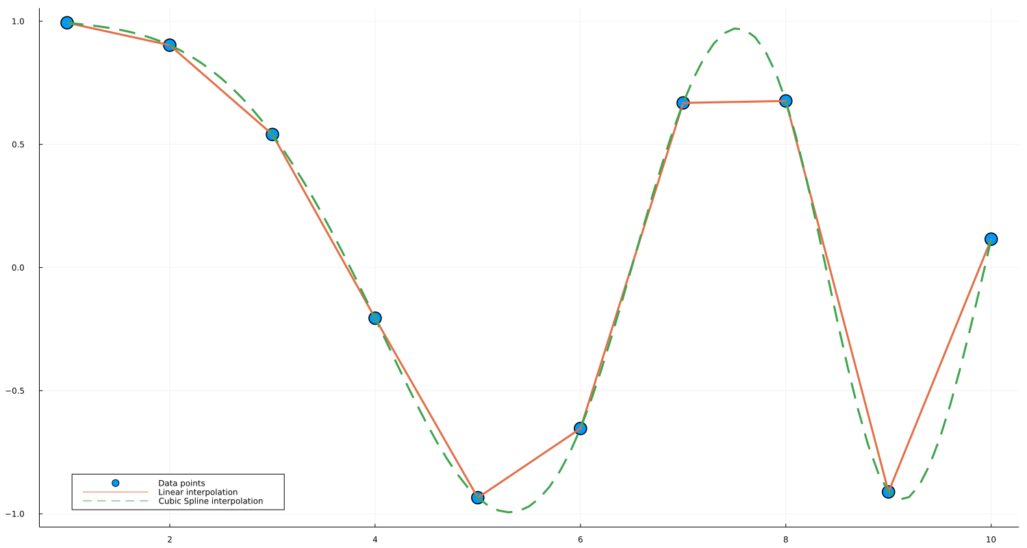
Example with Plots.jl
An interpolated object is also easily capable of being plotted with Plots.jl. A simple example is as follows:
using Interpolations, Plots

# Lower and higher bound of interval
a = 1.0
b = 10.0
# Interval definition
x = a:1.0:b
# This can be any sort of array data, as long as
# length(x) == length(y)
y = @. cos(x^2 / 9.0) # Function application by broadcasting
# Interpolations
itp_linear = linear_interpolation(x, y)
itp_cubic = cubic_spline_interpolation(x, y)
# Interpolation functions
f_linear(x) = itp_linear(x)
f_cubic(x) = itp_cubic(x)
# Plots
width, height = 1500, 800 # not strictly necessary
x_new = a:0.1:b # smoother interval, necessary for cubic spline

scatter(x, y, markersize=10,label="Data points")
plot!(f_linear, x_new, w=3,label="Linear interpolation")
plot!(f_cubic, x_new, linestyle=:dash, w=3, label="Cubic Spline interpolation")
plot!(size = (width, height))
plot!(legend = :bottomleft)
And the generated plot is: