Control of interpolation algorithm
BSplines
The interpolation type is described in terms of degree and, if necessary, boundary conditions. There are currently four degrees available: Constant, Linear, Quadratic, and Cubic corresponding to B-splines of degree 0, 1, 2, and 3 respectively.
B-splines of quadratic or higher degree require solving an equation system to obtain the interpolation coefficients, and for that you must specify a boundary condition that is applied to close the system. The following boundary conditions are implemented: Flat, Line (alternatively, Natural), Free, Periodic and Reflect; their mathematical implications are described in detail in their docstrings. When specifying these boundary conditions you also have to specify whether they apply at the edge grid point (OnGrid()) or beyond the edge point halfway to the next (fictitious) grid point (OnCell()).
Some examples:
# Nearest-neighbor interpolation
itp = interpolate(a, BSpline(Constant()))
v = itp(5.4)   # returns a[5]

# Previous-neighbor interpolation
itp = interpolate(a, BSpline(Constant(Previous)))
v = itp(1.8)   # returns a[1]

# Next-neighbor interpolation
itp = interpolate(a, BSpline(Constant(Next)))
v = itp(5.4)   # returns a[6]

# (Multi)linear interpolation
itp = interpolate(A, BSpline(Linear()))
v = itp(3.2, 4.1)  # returns 0.9*(0.8*A[3,4]+0.2*A[4,4]) + 0.1*(0.8*A[3,5]+0.2*A[4,5])

# Quadratic interpolation with reflecting boundary conditions
# Quadratic is the lowest order that has continuous gradient
itp = interpolate(A, BSpline(Quadratic(Reflect(OnCell()))))

# Linear interpolation in the first dimension, and no interpolation
# (just lookup) in the second
itp = interpolate(A, (BSpline(Linear()), NoInterp()))
v = itp(3.65, 5)  # returns  0.35*A[3,5] + 0.65*A[4,5]
There are more options available, for example:
# In-place interpolation
itp = interpolate!(A, BSpline(Quadratic(InPlace(OnCell()))))
which destroys the input A but also does not need to allocate as much memory.
Scaled BSplines
BSplines assume your data is uniformly spaced on the grid 1:N, or its multidimensional equivalent. If you have data of the form [f(x) for x in A], you need to tell Interpolations about the grid A. If A is not uniformly spaced, you must use gridded interpolation described below. However, if A is a collection of ranges or linspaces, you can use scaled BSplines. This is more efficient because the gridded algorithm does not exploit the uniform spacing. Scaled BSplines can also be used with any spline degree available for BSplines, while gridded interpolation does not currently support quadratic or cubic splines.
Some examples,
A_x = 1.:2.:40.
A = [log(x) for x in A_x]
itp = interpolate(A, BSpline(Cubic(Line(OnGrid()))))
sitp = scale(itp, A_x)
sitp(3.) # exactly log(3.)
sitp(3.5) # approximately log(3.5)
For multidimensional uniformly spaced grids
A_x1 = 1:.1:10
A_x2 = 1:.5:20
f(x1, x2) = log(x1+x2)
A = [f(x1,x2) for x1 in A_x1, x2 in A_x2]
itp = interpolate(A, BSpline(Cubic(Line(OnGrid()))))
sitp = scale(itp, A_x1, A_x2)
sitp(5., 10.) # exactly log(5 + 10)
sitp(5.6, 7.1) # approximately log(5.6 + 7.1)
Gridded interpolation
These use a very similar syntax to BSplines, with the major exception being that one does not get to choose the grid representation (they are all OnGrid). As such one must specify a set of coordinate arrays defining the nodes of the array.
In 1D
A = rand(20)
A_x = 1.0:2.0:40.0
nodes = (A_x,)
itp = interpolate(nodes, A, Gridded(Linear()))
itp(2.0)
The spacing between adjacent samples need not be constant; indeed, if they are constant, you'll get better performance with scaled.
The general syntax is
itp = interpolate(nodes, A, options...)where nodes = (xnodes, ynodes, ...) specifies the positions along each axis at which the array A is sampled for arbitrary ("rectangular") samplings.
For example:
A = rand(8,20)
nodes = ([x^2 for x = 1:8], [0.2y for y = 1:20])
itp = interpolate(nodes, A, Gridded(Linear()))
itp(4,1.2)  # approximately A[2,6]
One may also mix modes, by specifying a mode vector in the form of an explicit tuple:
itp = interpolate(nodes, A, (Gridded(Linear()), Gridded(Constant())))Presently there are only three modes for gridded:
- For linear interpolation between nodes
Gridded(Linear()) - For nearest neighbor interpolation on the applied axis
Gridded(Constant()) - For no interpolation. The coordinate of the selected input vector MUST be located on a grid point. Requests for off grid coordinates results in the throwing of an error.
NoInterp()
For Constant there are additional parameters. Use Constant{Previous}() in order to perform a previous neighbor interpolation. Use Constant{Next}() for a next neighbor interpolation. Note that rounding can be an issue, see issue #473.
missing data will naturally propagate through the interpolation, where some values will become missing. To avoid that, one can filter out the missing data points and use a gridded interpolation. For example:
x = 1:6
A = [i == 3 ? missing : i for i in x]
xf = [xi for (xi,a) in zip(x, A) if !ismissing(a)]
Af = filter(!ismissing, A)
itp = interpolate((xf, ), Af, Gridded(Linear()))
In-place gridded interpolation is also possible:
x = 1:4
y = view(rand(4), :)
itp = interpolate!((x,), y, Gridded(Linear()))
y .= 0
itp(2.5)0.0Parametric splines
Given a set a knots with coordinates x(t) and y(t), a parametric spline S(t) = (x(t),y(t)) parametrized by t in [0,1] can be constructed with the following code adapted from a post by Tomas Lycken:
using Interpolations

t = 0:.1:1
x = sin.(2π*t)
y = cos.(2π*t)
A = hcat(x,y)

itp = Interpolations.scale(
    interpolate(A, (BSpline(Cubic(Natural(OnGrid()))), NoInterp())),
    t,
    1:2
)

tfine = 0:.01:1
xs, ys = [itp(t,1) for t in tfine], [itp(t,2) for t in tfine]
We can then plot the spline with:
using Plots

scatter(x, y, label="knots")
plot!(xs, ys, label="spline")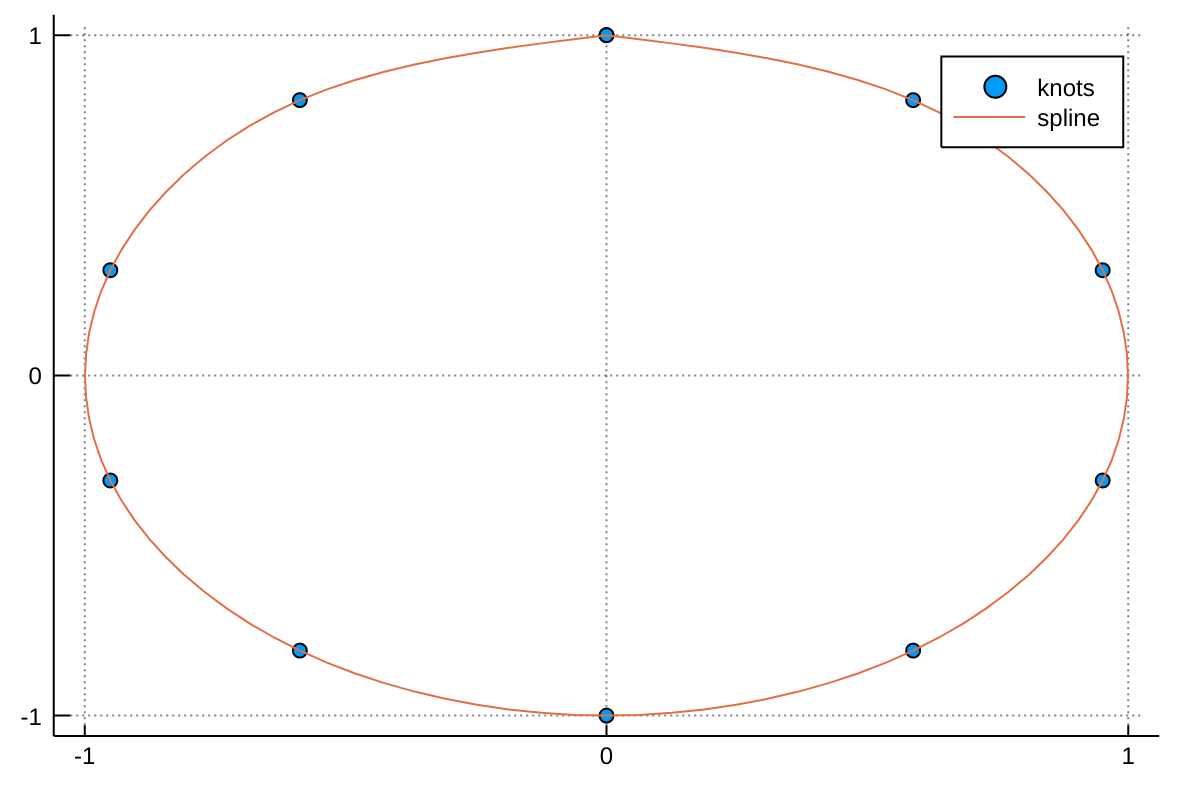
Monotonic interpolation
When you have some one-dimensional data that is monotonic, many standard interpolation methods may give an interpolating function that it is not monotonic. Monotonic interpolation ensures that the interpolating function is also monotonic.
Here is an example of making a cumulative distribution function for some data:
percentile_values = [
    0.0, 0.01, 0.1, 1.0, 2.0, 3.0, 4.0, 5.0, 6.0, 7.0, 8.0, 9.0,
    10.0, 20.0, 30.0, 40.0, 50.0, 60.0, 70.0, 80.0, 90.0,
    91.0, 92.0, 93.0, 94.0, 95.0, 96.0, 97.0, 98.0, 99.0,
    99.9, 99.99, 100.0
];

y = sort(randn(length(percentile_values))); # some random data

itp_cdf = extrapolate(
    interpolate(y, percentile_values, SteffenMonotonicInterpolation()),
    Flat()
);

t = -3.0:0.01:3.0 # just a range for calculating values of the interpolating function

interpolated_cdf = map(itp_cdf, t) # interpolating the CDF
There are a few different monotonic interpolation algorithms. Some guarantee that for non-monotonic data the interpolating function does not exceed the range of values between two successive points while other do not (this is called overshooting in the list below).
LinearMonotonicInterpolation– simple linear interpolation. Does not overshoot.FiniteDifferenceMonotonicInterpolation– it may overshoot.CardinalMonotonicInterpolation– it may overshoot.FritschCarlsonMonotonicInterpolation– it may overshoot.FritschButlandMonotonicInterpolation– it does not overshoot.SteffenMonotonicInterpolation– it does not overshoot.
You can read about monotonic interpolation in the following sources:
- Fritsch, F. N. and Butland, J. (1984). A Method for Constructing Local Monotone Piecewise Cubic Interpolants. SIAM Journal on Scientific and Statistical Computing 5, 300–304.
- Fritsch, F. N. and Carlson, R. E. (1980). Monotone Piecewise Cubic Interpolation. SIAM Journal on Numerical Analysis 17, 238–246.
- Steffen, M. (1990). A Simple Method for Monotonic Interpolation in One Dimension. Astronomy and Astrophysics 239, 443–450.