Accuracy and Parameters
The NFFT approximates the NDFT; its error depends on the window function $\varphi$, the window width $W$ (in grid points) and the oversampling factor $\sigma$ (see Mathematical Background). NFFT.jl lets you state the error you need and chooses these three for you.
From reltol to parameters
reltol is the requested relative error in the $\ell^2$ norm, for any nodes and data. For each combination of window family, $W$ and $\sigma$ NFFT.jl carries a table with the optimised shape parameter of the window and a bound on its aliasing error that also holds for nodes on grid points (Cartesian sampling, where the aliases of all nodes add up coherently). From all entries whose predicted error is below reltol, the plan takes the one with the lowest predicted run time. The cost model weighs the resampling ($J W^D$) against the FFT ($\sigma^D |\bm{N}| \log$), so the choice depends on the dimension and on the ratio of nodes to grid size. Plans on a GPU use a cost model of their own (see Parameter choice on a GPU).
using NFFT, LinearAlgebra, Random, CairoMakie
Random.seed!(1)

N = (48, 48)
k = rand(2, 4000) .- 0.5
f = randn(ComplexF64, N)
exact = NDFTPlan(k, N) * f
relerr(p) = norm(p * f - exact) / norm(exact)

p = plan_nfft(k, N; reltol=1e-6)
NFFTPlan{Float64} of size (48, 48) along dims 1:2 at 4000 nodes: ExpSemicircle window, W = 8, σ = 1.85, predicted error 7.200297966955764e-7The plan shows what it chose; NFFT.parameters returns the same as a named tuple:
NFFT.parameters(p)(window = ExpSemicircle(), W = 8, σ = 1.85)Over a range of tolerances, the measured error stays below the requested one and below accuracy(p), the bound the plan predicts:
tols = [10.0^-i for i in 2:13]
plans = [plan_nfft(k, N; reltol=t) for t in tols]
measured = relerr.(plans)
predicted = accuracy.(plans)

fig = Figure(size=(640, 380))
ax = Axis(fig[1, 1]; xscale=log10, yscale=log10, xreversed=true,
          xlabel="requested reltol", ylabel="relative error",
          xticks=LogTicks(-14:2:-2), yticks=LogTicks(-14:2:-2))
lines!(ax, tols, tols; color=:gray60, linestyle=:dash, label="reltol")
scatterlines!(ax, tols, predicted; label="accuracy(p)")
scatterlines!(ax, tols, measured; label="measured")
axislegend(ax; position=:rt)
fig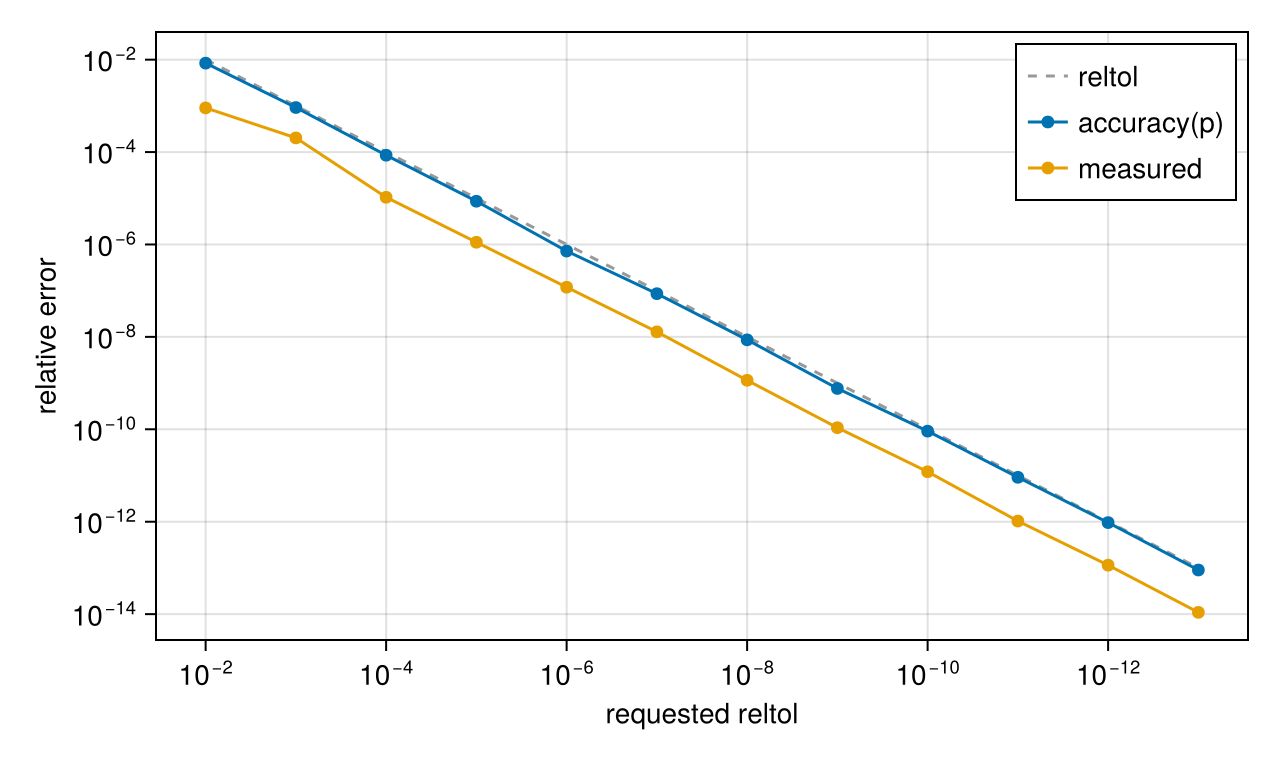
The chosen widths and oversampling factors:
[(reltol=t, W=NFFT.parameters(q).W, σ=NFFT.parameters(q).σ) for (t, q) in zip(tols, plans)]12-element Vector{@NamedTuple{reltol::Float64, W::Int64, σ::Float64}}:
(reltol = 0.010000000000000002, W = 5, σ = 1.3)
(reltol = 0.001, W = 5, σ = 1.6)
(reltol = 0.0001, W = 7, σ = 1.5)
(reltol = 1.0e-5, W = 8, σ = 1.5)
(reltol = 1.0e-6, W = 8, σ = 1.85)
(reltol = 1.0000000000000001e-7, W = 9, σ = 1.85)
(reltol = 1.0e-8, W = 10, σ = 1.9)
(reltol = 1.0e-9, W = 11, σ = 1.95)
(reltol = 1.0e-10, W = 12, σ = 1.95)
(reltol = 1.0e-11, W = 13, σ = 2.0)
(reltol = 1.0000000000000002e-12, W = 14, σ = 2.0)
(reltol = 1.0e-13, W = 14, σ = 2.45)Below about $10^{-13}$ rounding errors dominate in double precision (more for large $N$: node positions are accurate to $\approx \varepsilon \max N$); in single precision the floor is about $3 \cdot 10^{-6}$. A reltol below what any parameters reach throws an ArgumentError instead of returning a less accurate plan, unless W and σ are both given. Without reltol a plan uses default_reltol of its element type: $10^{-8}$, in single precision $1.2 \cdot 10^{-5}$.
Element types wider than Float64 (Double64 from DoubleFloats.jl, Float128 from Quadmath.jl) compute the window fit, the correction factors and the grid positions in their own precision and, with an FFT for them (fft = FFTABackend()), reach correspondingly smaller errors: reltol = 1e-25 with Double64 gives about $10^{-26}$, 1e-28 with Float128 about $10^{-29}$. Beyond the table ($W > 16$) the plan uses the Kaiser–Bessel window with $\beta = \pi W (1 - 1/(2\sigma))$, up to $W = 40$. The resampling kernels are unrolled in $W$: with Double64 and $W \approx 30$ in 2D the first transform compiles for minutes. The FFT of FFTA.jl loses accuracy with the length (up to $0.3 \, n \varepsilon$); the predicted error accounts for it.
Window families
Two families have parameter tables:
KaiserBessel: the continuous Kaiser–Bessel window,ExpSemicircle: the "exponential of semicircle" window $\exp(\beta((1-(2z/W)^2)^{e_0} - 1))$.
The default window = :auto lets both compete. How the error falls with the width, at $\sigma = 2$ and $\sigma = 1.25$:
Ws = 4:14
fig = Figure(size=(640, 380))
ax = Axis(fig[1, 1]; yscale=log10, xlabel="window width W", ylabel="relative error",
          xticks=Ws, yticks=LogTicks(-14:2:-2))
for (σ, style) in ((2.0, :solid), (1.25, :dash)), (win, name) in ((KaiserBessel(), "Kaiser–Bessel"),
                                                                   (ExpSemicircle(), "ES"))
  errs = [relerr(plan_nfft(k, N; window=win, W, σ)) for W in Ws]
  scatterlines!(ax, Ws, errs; linestyle=style, label="$name, σ = $σ")
end
axislegend(ax; position=:lb)
fig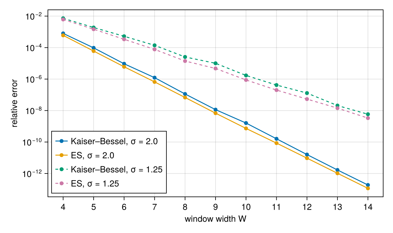
A smaller $\sigma$ needs a wider window for the same error, but its FFT is cheaper; which is faster overall depends on $D$ and on the number of nodes. This is the trade-off the automatic choice makes.
To set window, width or oversampling yourself, see Choosing Parameters; all plan options are listed in the API.
This page was generated using Literate.jl.