
Solving Poisson's equation with the DST
Find
The test problem has a known answer,
using FFTL, CairoMakie, LinearAlgebraThe eigenvalues of the 1D second difference with Dirichlet conditions are
function poisson_solve(n)
  h = 1 / (n + 1)
  x = [i * h for i in 1:n]
  uex = [sin(π * xi) * sin(2π * yj) for xi in x, yj in x]
  f = 5π^2 .* uex

  λ1 = [(2 - 2cos(j * π * h)) / h^2 for j in 1:n]
  Λ = [λ1[j] + λ1[k] for j in 1:n, k in 1:n]

  F = FFTL.r2r(f, (FFTL.RODFT00, FFTL.RODFT00), (1, 2))
  F ./= Λ
  u = FFTL.r2r(F, (FFTL.RODFT00, FFTL.RODFT00), (1, 2))
  u ./= (2 * (n + 1))^2
  u, uex
end

function poisson_error(n)
  u, uex = poisson_solve(n)
  maximum(abs, u - uex)
end
poisson_error (generic function with 1 method)Halving the grid spacing should divide the error by four (second order):
errs = [poisson_error(n) for n in (31, 63, 127)]
for (n, e) in zip((31, 63, 127), errs)
  println("n = ", n, ", max error ", round(e; sigdigits = 3))
end
println("ratios: ", round.(errs[1:end-1] ./ errs[2:end]; digits = 2))
n = 31, max error 0.00273
n = 63, max error 0.000683
n = 127, max error 0.000171
ratios: [4.0, 4.0]The numerical solution for n = 63, next to the convergence over a wider range of grid sizes against the slope-two guide:
u, uex = poisson_solve(63)
nvec = (15, 31, 63, 127, 255)
h = [1 / (n + 1) for n in nvec]
errs = [poisson_error(n) for n in nvec]

fig = Figure(size = (760, 330))
ax1 = Axis(fig[1, 1]; title = "solution, n = 63")
hidedecorations!(ax1)
heatmap!(ax1, u)
ax2 = Axis(fig[1, 2]; xscale = log10, yscale = log10, xlabel = "grid spacing h",
           ylabel = "max error")
scatter!(ax2, h, errs)
lines!(ax2, h, errs)
lines!(ax2, h, errs[1] .* (h ./ h[1]) .^ 2; linestyle = :dash, color = :gray,
       label = "slope 2")
axislegend(ax2; position = :rt)
fig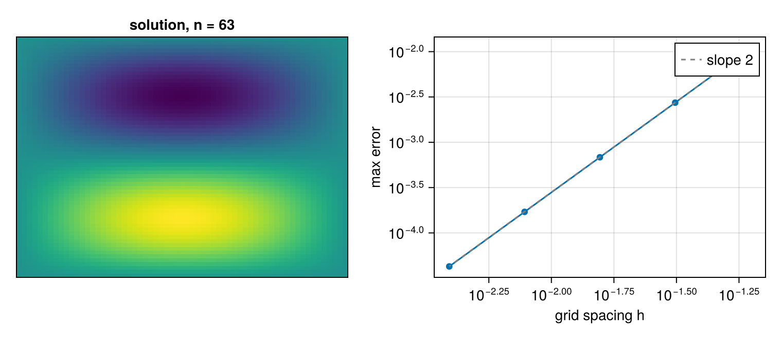
The scaling
The DST-I applied twice multiplies by FFTL.r2r does not normalise, so this factor is part of the algorithm, not of the library. The cosine, sine and Hartley how-to lists the factor for each kind.
This page was generated using Literate.jl.